Modeling

I use mathematical models to contextualize and interpret our geophysical measurements. Most of my modeling work has focused on developing theory for a specific physical process rather than in forecasting. Here, I try to provide some context for how I think about the physics of earth systems, but see the associated publications for a more detailed background.

Nondimensional Numbers

Physics problems are commonly ’nondimensionalized’ in order to compare the scale of two processes. As an example, take the Peclet number which compares thermal advection (convection) to thermal diffusion (conduction) in a moving fluid,

$$ Pe = \frac{vL}{\alpha} $$

where $ v $ is the fluid velocity, $ L $ is the characteristic length scale, and $ \alpha $ is the thermal diffusivity (a material constant). In a diffusion-dominated system, the thermal diffusivity is larger than the velocity time length scale, so $ Pe < 1 $ , as is the case in microfluidics with a slow-moving non-turbulent fluid moving through a small channel. Fluid systems are more commonly advection dominated, especially in Earth science applications, think river, ocean current, or even ice stream, with $ Pe \gg 1 $ .

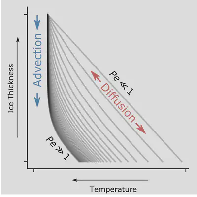
Ice sheets are generally advection dominated, but the scale varies depending on the setting. Take an ice divide, where flow is downward at ~0.1 m/yr and ice is ~2 km thick, then in the vertical $ Pe $ ~ 1-10, only slightly favoring advection. Thinking instead in the horizontal, across the spatial scales of an ice sheet, diffusion is entirely ineffective. Ice streams flow at ~100-1000 m/yr across effective length scales of many ice thicknesses, say 10-50 km, then in the horizontal $ Pe $ ~ 10⁴-10⁶. In cases like this, where the nondimensional number is very far from 1, processes can be ignored entirely often simplifying modeling or engineering applications.

In an ice-stream shear margin, there are four critical processes which control ice temperature: diffusion, vertical advection associated with new snow deposited at the surface, heat generation from the friction in plane shear, and downstream or cross-margin advection sourcing cold ice from outside the shear margin. The first two processes are compared using the standard $ Pe $ number which in this case (as above) is larger than 1 but only slightly. With the third process we introduce a new dimensionless number, the Brinkmann number which compares heat generation to diffusion,

$$ Br = \frac{QH^2}{k\Delta T} $$

These are generally large in an ice-stream shear margin, so much that without considering any other processes the shear margin would be mostly temperate ice. However, we know that cold ice is constantly moving through the system. We nondimensionalize this through a horizontal Peclet-like number

$$ \Lambda = \frac{H}{\alpha \Delta T} \int_0^H u \frac{\partial T}{\partial x} dz $$

We found that in a shear margin at Antarctica’s Siple Coast $ Br $ is only slightly larger than $ \Lambda $ , so ice temperatures should be warmer than the surrounding ice but not necessarily temperate.

Phase-Boundary Problems

One of the reasons the water molecule is so interesting is that both the melting point and the boiling point are within our range of experienced temperatures. Studying the transition between phases, in particular the ice-water transition, leads us to track how the boundary moves in time. Mathematical models which simulate these conditions solve the so-called Stefan problem which has another nondimensional number, the Stefan number,

$$ St = \frac{c\Delta T}{L} $$

where sensible heat (heat capacity, $c$, times the temperature gradient, $\Delta T$), is compared to latent heat ($L$). When $St\gg1$ heat is rapidly supplied to the phase boundary, so it moves quickly. When $ St\ll1$ the phase boundary is not supplied with sufficient energy to transition, so it moves slowly.

In a slightly more complicated scenario solute is introduced to the liquid, suppressing the melting point at the phase boundary. We call this an ’extended’ Stefan problem. Here, not only does heat need to be evacuated from the phase boundary for the freezing front to step forward, but solute also needs to be rejected from the fluid. Generally, rates of solute diffusion are much slower than thermal diffusion, so it becomes a dominant process. The two diffusion rates are compared with the Lewis number,

$$ Le = \frac{\alpha}{D} $$

where representative length scales for diffusion are $\sqrt{\alpha t}$ for thermal and $\sqrt{D t}$ for molecular diffusion of the solute.

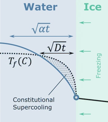
An example where both thermal and solute diffusion are at play is in sea-ice formation where ice freezes at the boundary between a cold atmosphere and a salty ocean. We applied this theory in cylindrical coordinates for refreezing of glacier boreholes when filled with an antifreeze solution.

Ice-Sheet Modeling

Most of my modeling work has been to isolate and explain physical processes, as above. However, a large component of the modeling community works to directly simulate the real-world behavior at the scale of an ice sheet.

As a collaboration with Dr. Matthew Hoffman of Los Alamos National Laboratory, I used the Model for Precision Across Scales (MPAS) to couple fluid flow beneath an ice sheet to the dynamics of the ice sheet itself. In essense, high pressure within the subglacial hydrologic system lifts the ice sheet off its substrate, allowing it to move faster. I have also done some work with Dr. Daniel Shapero on his finite-element ice-sheet model icepack. We are interested in simulating how ice dynamics effect the development of ice temperature and crystal orientation fabric.